第 7 章 回归
我们听过无数的道理,却仍旧过不好这一生。后会无期
Angrist在Most Harmless Econometrics写到:
Now we too spend our days happily perusing regression output, in the manner of our teaches and advisers in college and graduate school.
作为一名经济学家或经济学的学生,我们不是在跑回归,就是在为回归做准备。你也许听了很多讲座,参加了不少暑期学校,花了几笔冤枉钱,(很可能还被我骗过钱),但你还是不会跑回归。大概率是你没有好好完成Wooldridge 的课后习题,或者没有搞清楚Angrist 那些写在脚注里面的看似显然的证明。
不用担心,相信我,等你学完本章,你依然不会跑回归,因为跑回归重要的不是知道写什么代码,而是知道统计原理,这是江湖骗子和经济学家的区别。
作为本书的核心贡献,本章的目的是帮读者提炼出回归与因果推断中最核心的理论以及读者经常遇到的坑,并以案例的形式介绍在R中如何实现相关操作。如果你读了本章之后,照猫画虎的复制了几段代码就去江湖上招摇撞骗,我会画个圈圈诅咒你的。所以,如果你没有继续自学Wooldridge和Angrist,请闭上眼睛,想一下我在祖国东海边给你画的圈。
7.2 因果推断的反事实框架
7.2.1 定义因果关系
在定义因果关系之前,我们必须清楚,目前主流的统计学工具中,只能定义两个变量线性的因果关系,即变量D与变量Y的因果关系。例如:人才流动对科研生产率、人才流动对合作网络、人才计划对人才流动,以及研发资助对企业创新等关系。
如果D是Y原因,那D与Y显著相关(相关系数显著地不为0),且D发生在Y之前。但这两个条件仅仅是必要而非充分条件。以海外科学家回国任教是否有利其科研生涯这个问题为例,D是回国与否的0-1变量,Y是科研产出(例如科技论文数量)。即使我们观察到D与Y之间显著正相关,我们依然无法断言回国有利于科学家的科研生涯。这是因为很可能选择回归任教的科学家本身就是那些科研潜力更强、更适应国内研究环境的科学家,因此他们本身就应该比留在国外的华人科学家发表更多的论文。 计量经济学中,有两个路径可以定义因果关系。一种是通过引入反事实项来定义因果关系(Angtist,参考文献),另一种则是控制通过其他其他因素不变定义回归中的因果关系(伍德里奇,参考文献)。本讲义中,我们将采用第一种路径,通过CEF的三个定理,其实这两种路径是等价的。
沿用前面的表示方法,我们假定实验D是一个0-1变量(读者不用担心这一简化失去一般性,Angrsit已经将其推广到了连续变量)。对于观测个体i而言,\(D_{i} = 1\) 表示其属于实验组,例如科学家i选择回国任教,\(D_{i} = 1\) 则表示其属于对照组。个体i的观测结果依赖于是否参与实验,用\(Y_{i}\)表示,则:
\[Y_{i} = \left\{\begin{aligned} Y_{1,i},\quad if \quad D_{i} = 1\\ Y_{0,i},\quad if \quad D_{i} = 0 \end{aligned} \right.\]
由于在现实世界中,完成论文之后讨论的结果然后完成之后
7.7 包含高维分类变量的回归
在固定效应回归中,固定效应以因子(factor)的形式加入回归方程中。R中的这个处理方式虽然让公式变的非常简洁,但在计算时,有N个分类的固定效应还是要先转化成为N-1个0-1变量(为什么是N-1个?),因此M个观测值的回归就对应了M*(N-1)维度的协方差矩阵。当N非常大时,协方差矩阵正定形式的求逆将会是一个运算量很大的工作,此时回归就遭遇了维度灾难。
为了克服维度灾难,R中需要使用高纬度固定效应回归方法,一般线性模型使用lfe包中的felm函数,广义线性模型使用alpaca包的feglm函数。
felm函数的回归方程以|将因子与其他变量进行分割,其他写法与lm一致。例如:
feglm函数的回归方程与felm相似,唯一不同的是,因子需要提前定义好,不能以factor函数方式加入,例如下面的代码展示了如何使用feglm拟合高纬固定效应logit回归,
library(alpaca)
data <- data %>%
  mutate(f = factor(f),
         g = factor(g))
mod2 <- feglm(y ~ x | f + g,binomial(link = "logit"),data)另外,stargazer函数支持felm的回归模型mod1,但不支持feglm的回归模型mod2。如果要格式化输出feglm的回归模型,建议使用texreg包。
7.8 formula (公式)对象
尽管formula不是R语言的基础类,但它构成了R语言进行统计分析的基础。formula直观地刻画了变量之间的关系。formula是独立于数据之外的对象,换句话说,我们可以针对不同的数据使用同一个公式。
7.8.1 公式的生成
使用~连接因变量y与自变量x便可定义一个简单的公式,y ~ x。~相当于数学公式中的=。如果在R中使用class函数查看公式的类型,会返回”formula”。例如:
## [1] "formula"~右边可以有多个变量,变量之间通过 + 连接,例如y ~ x + z。
7.8.2 生成公式的运算符
R语言还有一些特殊运算符来方便地生成公式,总结如下表:
| 运算符 | 含义 | 例子 |
|---|---|---|
| + | 连接多个变量,说明有多个自变量 | y ~ x1 + x2 |
| . | 表示使用所有的变量 | y ~ . |
| : | 变量之间的交集 | y ~ x1 : x2 |
| * | 变量以及它们之间的交互 | y ~ x1 * x2 |
| ^ | 变量及n个变量之间的交互 | y ~ (x1 + x2)^2 |
| | | 在给定x2的条件下处理x1 | y ~ x1 |
| I() | 按照括号中的表达式进行算术表达式的处理 | y ~ x1 + I(x1^2) |
| log() | 数学函数也可以用在formula中 | log(y) ~ x1 + x2 |
| factor() | 将变量转换为因子 | y ~ x1 + factor(x2) |
| - | 表示排除某个变量 | y ~ x1 - x2 |
其中比较常用的包括,:,*和|。特别地,公式中使用x1:x2来表示交互项,而x1*x2并不是表示x1与x2的交互项,而是表示x1 + x2 + x1:x2。如果我们非要使用*来表达交互含义,则需要使用I运算符将公式写为,I(x1*x2)。|则被用于两阶段回归与高维数据回归中。
公式中还可以直接使用函数来对数据进行转换,常用的转换包括,使用log()将变量对数化,以及使用factor()函数将变量转换为因子(即研究设计中的分类变量)。
7.8.3 公式与字符串之间的转换
使用as.formula函数可以将符合要求的字符串转换为公式,例如:
## [1] "formula"需要注意的是,使用as.character函数无法将公式直接转化为对应的字符串,需要使用paste0函数对结果进行拼接。
## [1] "~" "y" "x + z"## [1] "y ~ x + z"当变量数据量很多的时候,可以先使用paste函数将相关变量粘贴成为一个字符串,然后再使用as.formula函数将字符串转化为公式,这样的操作可以让代码更加简洁。例如,
## y ~ x1 + x2 + x3 + x4 + x5 + x6 + x7 + x8 + x9 + x10 + x11 +
##     x12 + x13 + x14 + x15 + x16 + x17 + x18 + x19 + x20 + x21 +
##     x22 + x23 + x24 + x25
7.9 表达式expression
当我们在R代码中写下y <- x + 1 时,如果变量x没有被赋值,这一局代码会报错为object 'x' not found。
这个时候,我们会希望有一种方式可以在不执行的情况下储存y <- x + 1这段代码本身。这样的功能可以给我们的代码设计带来极大的方便。实现这一功能的对象便是表达式。
狭义上说,表达式是R里的一类特殊的对象(向量),它被用于储存一个完整的可独立执行的R语言语句。广义上讲,R语言的底层就是有这样的表达式组成的,了解表达式在R语言的中的灵活应用属于R语言高级编程的内容,读者可以参考大神Hadley Wickham的Advanced R1作进一步了解。
7.10 表达式的生成与执行
在R基本包中,可以使用expression函数生成一个表达式,以及使用eval函数执行相应的表达式。例如:
如果要判断一个对象是否是表达式,可以使用is.expression函数。例如:
## [1] TRUE7.11 表达式与字符串的转换
parse函数可以实现从字符串到表达式的转换,这会让我们对表达式的操作更加灵活。parse函数最重要的参数是text,即被转换的字符串。另一个重要的参数是encoding,被用于指定字符串的编码方式。
## [1] TRUE而parse函数的反函数是deparse,用于将表达式转换成字符串,例如:
MATHMATICAL ANNOTATION
https://stat.ethz.ch/R-manual/R-devel/library/grDevices/html/plotmath.html
7.12 使用stargazer输出表格
上一节中我们介绍了在R中如何拟合常见的回归模型。在实际的经济学研究中,拟合回归模型仅仅完成了回归分析一半的工作量,我们至少还需要花同样的时间将回归结果整理成正式发表(或投稿)论文中的标准回归表格式。初学者往往人工整理回归结果,这不仅与我们数据工程的自动化原则相违背,更重要的是,一旦在研究中对回归结果进行调整(这几乎是百分之百会发生的),人工整理将会耗费大量的时间与精力。
本节我们将介绍如何使用stargazer包输出回归结果表。stargazer2是政治经济学家 Marek Hlavac博士在哈佛大学肯尼迪学院攻读博士学位期间完成的包,已成为目前最流行的R包之一。stargazer可以将R的回归模型编码为html代码,LaTex代码或者是ASCII文本,将回归模型输出为可发表格式。除此之外,stargazer也可以输出描述性统计表,或者直接输出data.frame。通过下列代码安装与加载stargazer:
7.12.1 标准回归表
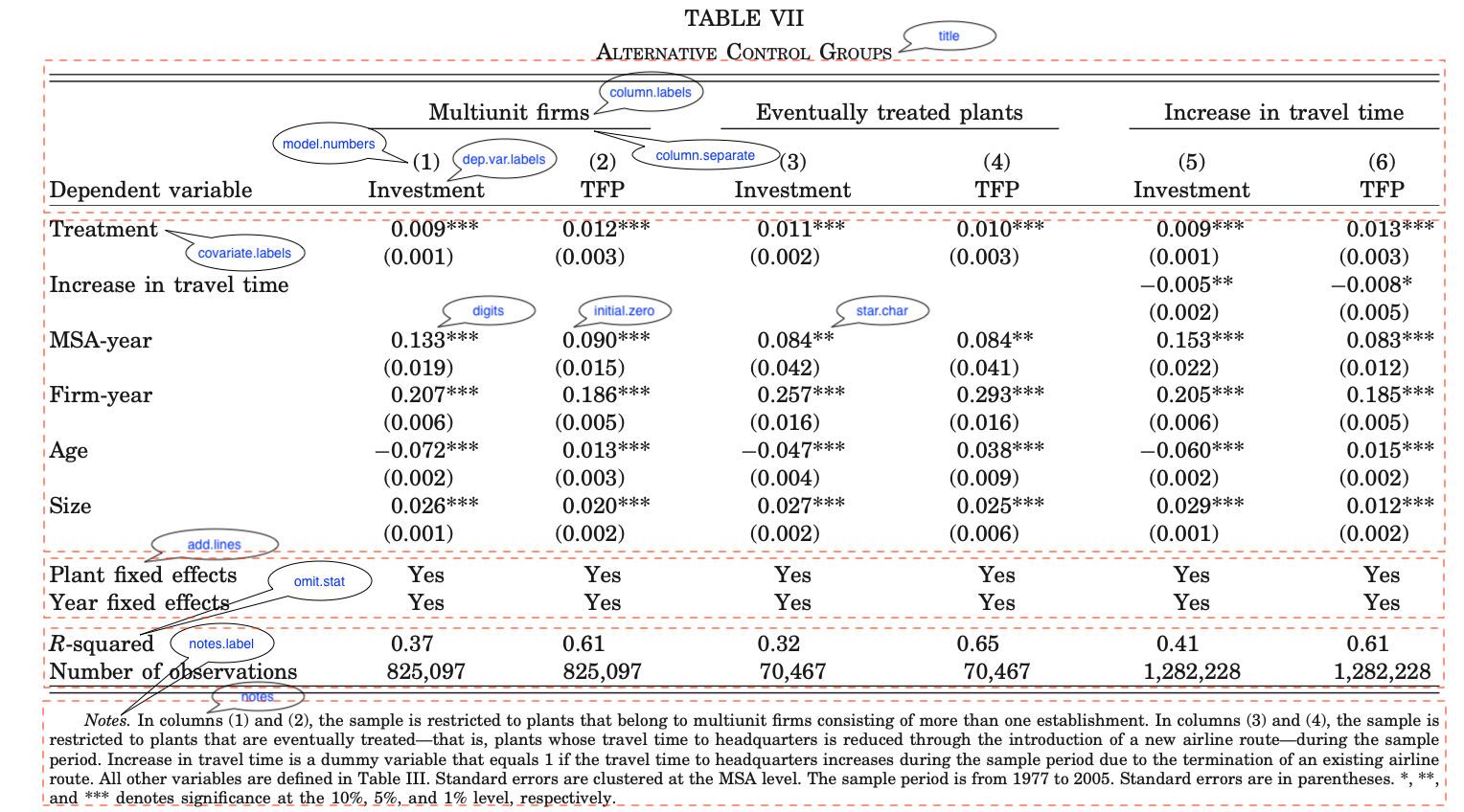
在学习使用stagazer之前,我们首先来看下正式发表论文的标准回归表。下表源自Giroud在The Quarterly Journal of Economics发表的论文Proximity and Investment: Evidence from Plant-Level Data3,我们可以发现,从上至下,标准回归表可以分为五个部分:第一部分包括因变量名、模型名以及模型编号;第二部分是自变量名与回归结果,包括回归系数、标准误差与显著性;第三部分是未汇报系数的变量;第三四部分是模型的统计指标;第五部分是注释。其中,第二部分是回归表的核心,而其他部分的重要性往往被初学者忽视。我们在回归表中标注了每一部分调整对应的stagazer中的参数,接下来我们将详细介绍各参数的使用方法。
7.12.2 默认格式
我们使用Wooldridge(2012)4 收录的JTRAIN数据集(详情见第十四章习题C3),该数据集源自Holzer等人(1993)5的劳动经济学论文,研究了工作培训津贴对于公司为雇员提供培训的作用。我们使用jtrain数据集拟合回归模型。
if(!require(wooldridge)){
  install.packages('wooldridge')
}
library(wooldridge)
library(stargazer)

data('jtrain')
names(jtrain)
## [1] "year" "fcode" "employ" "sales" "avgsal" "scrap"
## [7] "rework" "tothrs" "union" "grant" "d89" "d88"
## [13] "totrain" "hrsemp" "lscrap" "lemploy" "lsales" "lrework"
## [19] "lhrsemp" "lscrap_1" "grant_1" "clscrap" "cgrant" "clemploy"
## [25] "clsales" "lavgsal" "clavgsal" "cgrant_1" "chrsemp" "clhrsemp"mod1 <- lm(hrsemp ~ grant + grant_1 + lemploy, data = jtrain)
mod2 <- lm(hrsemp ~ grant + grant_1 + lemploy + union, data = jtrain)
mod3 <- lm(hrsemp ~ grant + grant_1 + lemploy + union + factor(fcode), data = jtrain)
mod4 <- lm(hrsemp ~ grant + grant_1 + lemploy + union + factor(fcode) + factor(year), data = jtrain)
mod5 <- glm(grant~lemploy + union, data = jtrain,family = binomial(link = "logit"))
# 在数据分析过程中,我们可以使用summary函数查看回归模型的结果
summary(mod1)##
## Call:
## lm(formula = hrsemp ~ grant + grant_1 + lemploy, data = jtrain)
##
## Residuals:
## Min 1Q Median 3Q Max
## -43.240 -11.641 -5.498 2.823 136.183
##
## Coefficients:
## Estimate Std. Error t value Pr(>|t|)
## (Intercept) 26.3527 4.0395 6.524 2.15e-10 ***
## grant 33.3370 3.1937 10.438 < 2e-16 ***
## grant_1 0.7895 4.0059 0.197 0.844
## lemploy -4.6289 1.0806 -4.283 2.33e-05 ***
## ---
## Signif. codes: 0 '***' 0.001 '**' 0.01 '*' 0.05 '.' 0.1 ' ' 1
##
## Residual standard error: 22.39 on 386 degrees of freedom
## (81 observations deleted due to missingness)
## Multiple R-squared: 0.2473, Adjusted R-squared: 0.2415
## F-statistic: 42.28 on 3 and 386 DF, p-value: < 2.2e-16在数据分析结束后,使用stargazer输出回归结果,stargazer定义了三种输出格式:html,LaTex和text,为方便我们使用html来做演示。
| Dependent variable: | |||
| hrsemp | grant | ||
| OLS | logistic | ||
| (1) | (2) | (3) | |
| grant | 33.337*** | 33.545*** | |
| (3.194) | (3.170) | ||
| grant_1 | 0.790 | 1.229 | |
| (4.006) | (3.979) | ||
| lemploy | -4.629*** | -3.892*** | 0.089 |
| (1.081) | (1.108) | (0.134) | |
| union | -7.734*** | 0.213 | |
| (2.925) | (0.332) | ||
| Constant | 26.353*** | 25.181*** | -2.155*** |
| (4.039) | (4.033) | (0.494) | |
| Observations | 390 | 390 | 440 |
| R2 | 0.247 | 0.261 | |
| Adjusted R2 | 0.241 | 0.253 | |
| Log Likelihood | -180.165 | ||
| Akaike Inf. Crit. | 366.331 | ||
| Residual Std. Error | 22.392 (df = 386) | 22.220 (df = 385) | |
| F Statistic | 42.280*** (df = 3; 386) | 33.949*** (df = 4; 385) | |
| Note: | p<0.1; p<0.05; p<0.01 | ||
stargazer内置了一些期刊风格的格式,可以使用style参数来指定,例如QJE的风格:
| hrsemp | grant | ||
| OLS | logistic | ||
| (1) | (2) | (3) | |
| grant | 33.337*** | 33.545*** | |
| (3.194) | (3.170) | ||
| grant_1 | 0.790 | 1.229 | |
| (4.006) | (3.979) | ||
| lemploy | -4.629*** | -3.892*** | 0.089 |
| (1.081) | (1.108) | (0.134) | |
| union | -7.734*** | 0.213 | |
| (2.925) | (0.332) | ||
| Constant | 26.353*** | 25.181*** | -2.155*** |
| (4.039) | (4.033) | (0.494) | |
| N | 390 | 390 | 440 |
| R2 | 0.247 | 0.261 | |
| Adjusted R2 | 0.241 | 0.253 | |
| Log Likelihood | -180.165 | ||
| Akaike Inf. Crit. | 366.331 | ||
| Residual Std. Error | 22.392 (df = 386) | 22.220 (df = 385) | |
| F Statistic | 42.280*** (df = 3; 386) | 33.949*** (df = 4; 385) | |
| Notes: | ***Significant at the 1 percent level. | ||
| **Significant at the 5 percent level. | |||
| *Significant at the 10 percent level. | |||
可以使用out参数将表格输出到文件
7.12.3 表格表头
通过title参数添加表格标题,通过dep.var.labels添加因变量标签,dep.var.caption设置因变量标题,默认情况也会输出模型名称。
stargazer(mod1, mod2, mod5, type = "html",
          title = "Table1: The empirical results",
dep.var.labels = c("Training hours","Training grants"))| Dependent variable: | |||
| Training hours | Training grants | ||
| OLS | logistic | ||
| (1) | (2) | (3) | |
| grant | 33.337*** | 33.545*** | |
| (3.194) | (3.170) | ||
| grant_1 | 0.790 | 1.229 | |
| (4.006) | (3.979) | ||
| lemploy | -4.629*** | -3.892*** | 0.089 |
| (1.081) | (1.108) | (0.134) | |
| union | -7.734*** | 0.213 | |
| (2.925) | (0.332) | ||
| Constant | 26.353*** | 25.181*** | -2.155*** |
| (4.039) | (4.033) | (0.494) | |
| Observations | 390 | 390 | 440 |
| R2 | 0.247 | 0.261 | |
| Adjusted R2 | 0.241 | 0.253 | |
| Log Likelihood | -180.165 | ||
| Akaike Inf. Crit. | 366.331 | ||
| Residual Std. Error | 22.392 (df = 386) | 22.220 (df = 385) | |
| F Statistic | 42.280*** (df = 3; 386) | 33.949*** (df = 4; 385) | |
| Note: | p<0.1; p<0.05; p<0.01 | ||
使用column.labels为回归结果添加列标签
stargazer(mod1, mod2, mod5, type = "html",
          title = "Table1: The empirical results",
          dep.var.labels = c("Training hours","Training grant"),
column.labels = c("Basic", "With union", "Selection"))| Dependent variable: | |||
| Training hours | Training grant | ||
| OLS | logistic | ||
| Basic | With union | Selection | |
| (1) | (2) | (3) | |
| grant | 33.337*** | 33.545*** | |
| (3.194) | (3.170) | ||
| grant_1 | 0.790 | 1.229 | |
| (4.006) | (3.979) | ||
| lemploy | -4.629*** | -3.892*** | 0.089 |
| (1.081) | (1.108) | (0.134) | |
| union | -7.734*** | 0.213 | |
| (2.925) | (0.332) | ||
| Constant | 26.353*** | 25.181*** | -2.155*** |
| (4.039) | (4.033) | (0.494) | |
| Observations | 390 | 390 | 440 |
| R2 | 0.247 | 0.261 | |
| Adjusted R2 | 0.241 | 0.253 | |
| Log Likelihood | -180.165 | ||
| Akaike Inf. Crit. | 366.331 | ||
| Residual Std. Error | 22.392 (df = 386) | 22.220 (df = 385) | |
| F Statistic | 42.280*** (df = 3; 386) | 33.949*** (df = 4; 385) | |
| Note: | p<0.1; p<0.05; p<0.01 | ||
多列结果共同使用同一个列标签,此时需要使用column.separate参数指定分割方法。
stargazer(mod1, mod2, mod5, type = "html",
          title = "Table1: The empirical results",
          dep.var.labels = c("Training hours","Training grant"),
          column.labels = c("Basic", "Selection"),
column.separate = c(2, 1))| Dependent variable: | |||
| Training hours | Training grant | ||
| OLS | logistic | ||
| Basic | Selection | ||
| (1) | (2) | (3) | |
| grant | 33.337*** | 33.545*** | |
| (3.194) | (3.170) | ||
| grant_1 | 0.790 | 1.229 | |
| (4.006) | (3.979) | ||
| lemploy | -4.629*** | -3.892*** | 0.089 |
| (1.081) | (1.108) | (0.134) | |
| union | -7.734*** | 0.213 | |
| (2.925) | (0.332) | ||
| Constant | 26.353*** | 25.181*** | -2.155*** |
| (4.039) | (4.033) | (0.494) | |
| Observations | 390 | 390 | 440 |
| R2 | 0.247 | 0.261 | |
| Adjusted R2 | 0.241 | 0.253 | |
| Log Likelihood | -180.165 | ||
| Akaike Inf. Crit. | 366.331 | ||
| Residual Std. Error | 22.392 (df = 386) | 22.220 (df = 385) | |
| F Statistic | 42.280*** (df = 3; 386) | 33.949*** (df = 4; 385) | |
| Note: | p<0.1; p<0.05; p<0.01 | ||
去除因变量标签、因变量标题、模型编码以及模型名称,当然实际应用中,不可能全部去除。
stargazer(mod1, mod2, mod5, type = "html",
          dep.var.caption = "",
          dep.var.labels.include = FALSE,
          model.numbers = FALSE,
model.names = FALSE)| grant | 33.337*** | 33.545*** | |
| (3.194) | (3.170) | ||
| grant_1 | 0.790 | 1.229 | |
| (4.006) | (3.979) | ||
| lemploy | -4.629*** | -3.892*** | 0.089 |
| (1.081) | (1.108) | (0.134) | |
| union | -7.734*** | 0.213 | |
| (2.925) | (0.332) | ||
| Constant | 26.353*** | 25.181*** | -2.155*** |
| (4.039) | (4.033) | (0.494) | |
| Observations | 390 | 390 | 440 |
| R2 | 0.247 | 0.261 | |
| Adjusted R2 | 0.241 | 0.253 | |
| Log Likelihood | -180.165 | ||
| Akaike Inf. Crit. | 366.331 | ||
| Residual Std. Error | 22.392 (df = 386) | 22.220 (df = 385) | |
| F Statistic | 42.280*** (df = 3; 386) | 33.949*** (df = 4; 385) | |
| Note: | p<0.1; p<0.05; p<0.01 | ||
7.12.4 表格正文
在mod3和mod4中我们逐步加入了所在企业与年份的固定效应,其中企业的固定效应包含了156个哑变量,我们不可能也不需要全部输出这些变量的回归系数。我们使用omit参数来确定不需要输出回归结果的变量。
stargazer(mod1, mod2, mod3,mod4,mod5,
          type = "html",
          dep.var.caption = "",
          column.labels = c("Basic","With Union","Factory","F&Y","Selection"),
          dep.var.labels = c("Training hours","Training grant"),
          model.names = FALSE,
omit = c("fcode","year"))| Training hours | Training grant | ||||
| Basic | With Union | Factory | F&Y | Selection | |
| (1) | (2) | (3) | (4) | (5) | |
| grant | 33.337*** | 33.545*** | 35.962*** | 34.228*** | |
| (3.194) | (3.170) | (2.509) | (2.858) | ||
| grant_1 | 0.790 | 1.229 | 5.664* | 0.504 | |
| (4.006) | (3.979) | (3.304) | (4.127) | ||
| lemploy | -4.629*** | -3.892*** | 1.755 | -0.176 | 0.089 |
| (1.081) | (1.108) | (4.102) | (4.288) | (0.134) | |
| union | -7.734*** | -5.150 | -5.060 | 0.213 | |
| (2.925) | (11.759) | (11.664) | (0.332) | ||
| Constant | 26.353*** | 25.181*** | -2.261 | 5.944 | -2.155*** |
| (4.039) | (4.033) | (21.238) | (21.698) | (0.494) | |
| Observations | 390 | 390 | 390 | 390 | 440 |
| R2 | 0.247 | 0.261 | 0.797 | 0.802 | |
| Adjusted R2 | 0.241 | 0.253 | 0.686 | 0.691 | |
| Log Likelihood | -180.165 | ||||
| Akaike Inf. Crit. | 366.331 | ||||
| Residual Std. Error | 22.392 (df = 386) | 22.220 (df = 385) | 14.400 (df = 252) | 14.283 (df = 250) | |
| F Statistic | 42.280*** (df = 3; 386) | 33.949*** (df = 4; 385) | 7.212*** (df = 137; 252) | 7.269*** (df = 139; 250) | |
| Note: | p<0.1; p<0.05; p<0.01 | ||||
进一步,我们可以通过covariate.labels参数来为自变量设定标签。
stargazer(mod1, mod2, mod3,mod4,mod5,
          type = "html",
          dep.var.caption = "",
          column.labels = c("Basic","With Union","Factory","F&Y","Selection"),
          dep.var.labels = c("Training hours","Training grant"),
          model.names = FALSE,
          omit = c("fcode","year"),
covariate.labels = c("Traning Grant", "Traning Grant 1 Year Before","log(Employment)","Labor Union"))| Training hours | Training grant | ||||
| Basic | With Union | Factory | F&Y | Selection | |
| (1) | (2) | (3) | (4) | (5) | |
| Traning Grant | 33.337*** | 33.545*** | 35.962*** | 34.228*** | |
| (3.194) | (3.170) | (2.509) | (2.858) | ||
| Traning Grant 1 Year Before | 0.790 | 1.229 | 5.664* | 0.504 | |
| (4.006) | (3.979) | (3.304) | (4.127) | ||
| log(Employment) | -4.629*** | -3.892*** | 1.755 | -0.176 | 0.089 |
| (1.081) | (1.108) | (4.102) | (4.288) | (0.134) | |
| Labor Union | -7.734*** | -5.150 | -5.060 | 0.213 | |
| (2.925) | (11.759) | (11.664) | (0.332) | ||
| Constant | 26.353*** | 25.181*** | -2.261 | 5.944 | -2.155*** |
| (4.039) | (4.033) | (21.238) | (21.698) | (0.494) | |
| Observations | 390 | 390 | 390 | 390 | 440 |
| R2 | 0.247 | 0.261 | 0.797 | 0.802 | |
| Adjusted R2 | 0.241 | 0.253 | 0.686 | 0.691 | |
| Log Likelihood | -180.165 | ||||
| Akaike Inf. Crit. | 366.331 | ||||
| Residual Std. Error | 22.392 (df = 386) | 22.220 (df = 385) | 14.400 (df = 252) | 14.283 (df = 250) | |
| F Statistic | 42.280*** (df = 3; 386) | 33.949*** (df = 4; 385) | 7.212*** (df = 137; 252) | 7.269*** (df = 139; 250) | |
| Note: | p<0.1; p<0.05; p<0.01 | ||||
为了突出我们关心的回归系数(coefficients of interest),我们可以使用order参数来调整自变量的排列顺序,注意此时变量标签也要做相应的调整,否则会导致结果出错。
stargazer(mod1, mod2, mod3,mod4,mod5,
          type = "html",
          dep.var.caption = "",
          column.labels = c("Basic","With Union","Factory","F&Y","Selection"),
          dep.var.labels = c("Training hours","Training grant"),
          model.names = FALSE,
          omit = c("fcode","year"),
          covariate.labels = c("log(Employment)","Labor Union","Traning Grant", "Traning Grant 1 Year Before"),
order = c(3, 4, 1, 2))| Training hours | Training grant | ||||
| Basic | With Union | Factory | F&Y | Selection | |
| (1) | (2) | (3) | (4) | (5) | |
| log(Employment) | -4.629*** | -3.892*** | 1.755 | -0.176 | 0.089 |
| (1.081) | (1.108) | (4.102) | (4.288) | (0.134) | |
| Labor Union | -7.734*** | -5.150 | -5.060 | 0.213 | |
| (2.925) | (11.759) | (11.664) | (0.332) | ||
| Traning Grant | 33.337*** | 33.545*** | 35.962*** | 34.228*** | |
| (3.194) | (3.170) | (2.509) | (2.858) | ||
| Traning Grant 1 Year Before | 0.790 | 1.229 | 5.664* | 0.504 | |
| (4.006) | (3.979) | (3.304) | (4.127) | ||
| Constant | 26.353*** | 25.181*** | -2.261 | 5.944 | -2.155*** |
| (4.039) | (4.033) | (21.238) | (21.698) | (0.494) | |
| Observations | 390 | 390 | 390 | 390 | 440 |
| R2 | 0.247 | 0.261 | 0.797 | 0.802 | |
| Adjusted R2 | 0.241 | 0.253 | 0.686 | 0.691 | |
| Log Likelihood | -180.165 | ||||
| Akaike Inf. Crit. | 366.331 | ||||
| Residual Std. Error | 22.392 (df = 386) | 22.220 (df = 385) | 14.400 (df = 252) | 14.283 (df = 250) | |
| F Statistic | 42.280*** (df = 3; 386) | 33.949*** (df = 4; 385) | 7.212*** (df = 137; 252) | 7.269*** (df = 139; 250) | |
| Note: | p<0.1; p<0.05; p<0.01 | ||||
使用digits可以指定小数点后保留的有效数位,使用initial.zero=FALSE可以去掉小数点前的无效数字0
stargazer(mod1, mod2, mod3,mod4,mod5,
          type = "html",
          dep.var.caption = "",
          column.labels = c("Basic","With Union","Factory","F&Y","Selection"),
          dep.var.labels = c("Training hours","Training grant"),
          model.names = FALSE,
          omit = c("fcode","year"),
          covariate.labels = c("log(Employment)","Labor Union","Traning Grant", "Traning Grant 1 Year Before"),
          order = c(3, 4, 1, 2),
          digits = 2,
initial.zero=FALSE)| Training hours | Training grant | ||||
| Basic | With Union | Factory | F&Y | Selection | |
| (1) | (2) | (3) | (4) | (5) | |
| log(Employment) | -4.63*** | -3.89*** | 1.76 | -.18 | .09 |
| (1.08) | (1.11) | (4.10) | (4.29) | (.13) | |
| Labor Union | -7.73*** | -5.15 | -5.06 | .21 | |
| (2.93) | (11.76) | (11.66) | (.33) | ||
| Traning Grant | 33.34*** | 33.55*** | 35.96*** | 34.23*** | |
| (3.19) | (3.17) | (2.51) | (2.86) | ||
| Traning Grant 1 Year Before | .79 | 1.23 | 5.66* | .50 | |
| (4.01) | (3.98) | (3.30) | (4.13) | ||
| Constant | 26.35*** | 25.18*** | -2.26 | 5.94 | -2.15*** |
| (4.04) | (4.03) | (21.24) | (21.70) | (.49) | |
| Observations | 390 | 390 | 390 | 390 | 440 |
| R2 | .25 | .26 | .80 | .80 | |
| Adjusted R2 | .24 | .25 | .69 | .69 | |
| Log Likelihood | -180.17 | ||||
| Akaike Inf. Crit. | 366.33 | ||||
| Residual Std. Error | 22.39 (df = 386) | 22.22 (df = 385) | 14.40 (df = 252) | 14.28 (df = 250) | |
| F Statistic | 42.28*** (df = 3; 386) | 33.95*** (df = 4; 385) | 7.21*** (df = 137; 252) | 7.27*** (df = 139; 250) | |
| Note: | p<0.1; p<0.05; p<0.01 | ||||
stargazer默认的显著性水平标记为p<0.1; p<0.05; p<0.01。有些时候我们需要调整显著性水平的标注标准,star.cutoffs参数可以实现这一调整。此外,star.char 参数可以修改显著性水平的标记。
stargazer(mod1, mod2, mod3,mod4,mod5,
          type = "html",
          dep.var.caption = "",
          column.labels = c("Basic","With Union","Factory","F&Y","Selection"),
          dep.var.labels = c("Training hours","Training grant"),
          model.names = FALSE,
          omit = c("fcode","year"),
          covariate.labels = c("log(Employment)","Labor Union","Traning Grant", "Traning Grant 1 Year Before"),
          order = c(3, 4, 1, 2),
          star.cutoffs = c(0.05,0.01,0.001),
star.char = c("†","*", "**"))| Training hours | Training grant | ||||
| Basic | With Union | Factory | F&Y | Selection | |
| (1) | (2) | (3) | (4) | (5) | |
| log(Employment) | -4.629** | -3.892** | 1.755 | -0.176 | 0.089 |
| (1.081) | (1.108) | (4.102) | (4.288) | (0.134) | |
| Labor Union | -7.734* | -5.150 | -5.060 | 0.213 | |
| (2.925) | (11.759) | (11.664) | (0.332) | ||
| Traning Grant | 33.337** | 33.545** | 35.962** | 34.228** | |
| (3.194) | (3.170) | (2.509) | (2.858) | ||
| Traning Grant 1 Year Before | 0.790 | 1.229 | 5.664 | 0.504 | |
| (4.006) | (3.979) | (3.304) | (4.127) | ||
| Constant | 26.353** | 25.181** | -2.261 | 5.944 | -2.155** |
| (4.039) | (4.033) | (21.238) | (21.698) | (0.494) | |
| Observations | 390 | 390 | 390 | 390 | 440 |
| R2 | 0.247 | 0.261 | 0.797 | 0.802 | |
| Adjusted R2 | 0.241 | 0.253 | 0.686 | 0.691 | |
| Log Likelihood | -180.165 | ||||
| Akaike Inf. Crit. | 366.331 | ||||
| Residual Std. Error | 22.392 (df = 386) | 22.220 (df = 385) | 14.400 (df = 252) | 14.283 (df = 250) | |
| F Statistic | 42.280** (df = 3; 386) | 33.949** (df = 4; 385) | 7.212** (df = 137; 252) | 7.269** (df = 139; 250) | |
| Note: | p<0.05; p<0.01; p<0.001 | ||||
7.12.5 添加变量信息
对于没有汇报的固定效应,我们需要手动添加相应信息,对于其他控制变量,我们可以选择在note中加以说明。
stargazer(mod1, mod2, mod3,mod4,mod5,
          type = "html",
          dep.var.caption = "",
          column.labels = c("Basic","With Union","Factory","F&Y","Selection"),
          dep.var.labels = c("Training hours","Training grant"),
          model.names = FALSE,
          omit = c("fcode","year"),
          covariate.labels = c("log(Employment)","Labor Union","Traning Grant", "Traning Grant 1 Year Before"),
          order = c(3, 4, 1, 2),
          add.lines = list(c("Factory FE", "No", "No","Yes","Yes","Yes"),
c("Year FE", "No", "No","No","Yes","Yes")))| Training hours | Training grant | ||||
| Basic | With Union | Factory | F&Y | Selection | |
| (1) | (2) | (3) | (4) | (5) | |
| log(Employment) | -4.629*** | -3.892*** | 1.755 | -0.176 | 0.089 |
| (1.081) | (1.108) | (4.102) | (4.288) | (0.134) | |
| Labor Union | -7.734*** | -5.150 | -5.060 | 0.213 | |
| (2.925) | (11.759) | (11.664) | (0.332) | ||
| Traning Grant | 33.337*** | 33.545*** | 35.962*** | 34.228*** | |
| (3.194) | (3.170) | (2.509) | (2.858) | ||
| Traning Grant 1 Year Before | 0.790 | 1.229 | 5.664* | 0.504 | |
| (4.006) | (3.979) | (3.304) | (4.127) | ||
| Constant | 26.353*** | 25.181*** | -2.261 | 5.944 | -2.155*** |
| (4.039) | (4.033) | (21.238) | (21.698) | (0.494) | |
| Factory FE | No | No | Yes | Yes | Yes |
| Year FE | No | No | No | Yes | Yes |
| Observations | 390 | 390 | 390 | 390 | 440 |
| R2 | 0.247 | 0.261 | 0.797 | 0.802 | |
| Adjusted R2 | 0.241 | 0.253 | 0.686 | 0.691 | |
| Log Likelihood | -180.165 | ||||
| Akaike Inf. Crit. | 366.331 | ||||
| Residual Std. Error | 22.392 (df = 386) | 22.220 (df = 385) | 14.400 (df = 252) | 14.283 (df = 250) | |
| F Statistic | 42.280*** (df = 3; 386) | 33.949*** (df = 4; 385) | 7.212*** (df = 137; 252) | 7.269*** (df = 139; 250) | |
| Note: | p<0.1; p<0.05; p<0.01 | ||||
7.12.6 选择统计量
在输出结果时,我们需要根据模型来选择汇报哪些统计量。stargazer使用omit.stat或者keep.stat来指定忽略或者保留的统计量。具体统计量的对应关系如下:
| 代码 | 统计量 |
|---|---|
| “all” | all statistics |
| “adj.rsq” | adjusted R-squared |
| “aic” | Akaike Information Criterion |
| “bic” | Bayesian Information Criterion |
| “chi2” | chi-squared |
| “f” | F statistic |
| “ll” | log-likelihood |
| “logrank” | score (logrank) test |
| “lr” | likelihood ratio (LR) test |
| “max.rsq” | maximum R-squared |
| “n” | number of observations |
| “null.dev” | null deviance |
| “Mills” | Inverse Mills Ratio |
| “res.dev” | residual deviance |
| “rho” | rho |
| “rsq” | R-squared |
| “scale” | scale |
| “theta” | theta |
| “ser” | standard error of the regression (i.e., residual standard error) |
| “sigma2” | sigma squared |
| “ubre” | Un-Biased Risk Estimator |
| “wald” | Wald test |
stargazer(mod1, mod2, mod3,mod4,mod5,
          type = "html",
          dep.var.caption = "",
          column.labels = c("Basic","With Union","Factory","F&Y","Selection"),
          dep.var.labels = c("Training hours","Training grant"),
          model.names = FALSE,
          omit = c("fcode","year"),
          covariate.labels = c("log(Employment)","Labor Union","Traning Grant", "Traning Grant 1 Year Before"),
          order = c(3, 4, 1, 2),
          add.lines = list(c("Factory FE", "No", "No","Yes","Yes","Yes"),
                           c("Year FE", "No", "No","No","Yes","Yes")),
keep.stat = c("n","ll","rsq","f"))| Training hours | Training grant | ||||
| Basic | With Union | Factory | F&Y | Selection | |
| (1) | (2) | (3) | (4) | (5) | |
| log(Employment) | -4.629*** | -3.892*** | 1.755 | -0.176 | 0.089 |
| (1.081) | (1.108) | (4.102) | (4.288) | (0.134) | |
| Labor Union | -7.734*** | -5.150 | -5.060 | 0.213 | |
| (2.925) | (11.759) | (11.664) | (0.332) | ||
| Traning Grant | 33.337*** | 33.545*** | 35.962*** | 34.228*** | |
| (3.194) | (3.170) | (2.509) | (2.858) | ||
| Traning Grant 1 Year Before | 0.790 | 1.229 | 5.664* | 0.504 | |
| (4.006) | (3.979) | (3.304) | (4.127) | ||
| Constant | 26.353*** | 25.181*** | -2.261 | 5.944 | -2.155*** |
| (4.039) | (4.033) | (21.238) | (21.698) | (0.494) | |
| Factory FE | No | No | Yes | Yes | Yes |
| Year FE | No | No | No | Yes | Yes |
| Observations | 390 | 390 | 390 | 390 | 440 |
| R2 | 0.247 | 0.261 | 0.797 | 0.802 | |
| Log Likelihood | -180.165 | ||||
| F Statistic | 42.280*** (df = 3; 386) | 33.949*** (df = 4; 385) | 7.212*** (df = 137; 252) | 7.269*** (df = 139; 250) | |
| Note: | p<0.1; p<0.05; p<0.01 | ||||
进一步,我们使用df = FALSE去掉自由度,这样的表格看上去就清爽多了。
stargazer(mod1, mod2, mod3,mod4,mod5,
          type = "html",
          dep.var.caption = "",
          column.labels = c("Basic","With Union","Factory","F&Y","Selection"),
          dep.var.labels = c("Training hours","Training grant"),
          model.names = FALSE,
          omit = c("fcode","year"),
          covariate.labels = c("log(Employment)","Labor Union","Traning Grant", "Traning Grant 1 Year Before"),
          order = c(3, 4, 1, 2),
          add.lines = list(c("Factory FE", "No", "No","Yes","Yes","Yes"),
                           c("Year FE", "No", "No","No","Yes","Yes")),
          keep.stat = c("n","ll","rsq","f"),
df = FALSE)| Training hours | Training grant | ||||
| Basic | With Union | Factory | F&Y | Selection | |
| (1) | (2) | (3) | (4) | (5) | |
| log(Employment) | -4.629*** | -3.892*** | 1.755 | -0.176 | 0.089 |
| (1.081) | (1.108) | (4.102) | (4.288) | (0.134) | |
| Labor Union | -7.734*** | -5.150 | -5.060 | 0.213 | |
| (2.925) | (11.759) | (11.664) | (0.332) | ||
| Traning Grant | 33.337*** | 33.545*** | 35.962*** | 34.228*** | |
| (3.194) | (3.170) | (2.509) | (2.858) | ||
| Traning Grant 1 Year Before | 0.790 | 1.229 | 5.664* | 0.504 | |
| (4.006) | (3.979) | (3.304) | (4.127) | ||
| Constant | 26.353*** | 25.181*** | -2.261 | 5.944 | -2.155*** |
| (4.039) | (4.033) | (21.238) | (21.698) | (0.494) | |
| Factory FE | No | No | Yes | Yes | Yes |
| Year FE | No | No | No | Yes | Yes |
| Observations | 390 | 390 | 390 | 390 | 440 |
| R2 | 0.247 | 0.261 | 0.797 | 0.802 | |
| Log Likelihood | -180.165 | ||||
| F Statistic | 42.280*** | 33.949*** | 7.212*** | 7.269*** | |
| Note: | p<0.1; p<0.05; p<0.01 | ||||
7.12.7 表格注释
回归表格的注释在经济学论文中是非常重要的。经济学中往往要求表格本身是可以被独立阅读和理解的,因此经济学家往往会在表格的注释中添加大量的补充信息,例如模型的细节,表格正文中未汇报的变量,甚至一些变量的测度方式等。stargaze的notes参数可以用来添加注释,同时通过notes.append = FALSE/TRUE来设定是否覆盖模型默认的note,notes.align用来设置note的对齐方式,notes.label则用于设置note的标签名。
stargazer(mod1, mod2, mod3,mod4,mod5,
          type = "html",
          dep.var.caption = "",
          column.labels = c("Basic","With Union","Factory","F&Y","Selection"),
          dep.var.labels = c("Training hours","Training grant"),
          model.names = FALSE,
          omit = c("fcode","year"),
          covariate.labels = c("log(Employment)","Labor Union","Traning Grant", "Traning Grant 1 Year Before"),
          order = c(3, 4, 1, 2),
          add.lines = list(c("Factory FE", "No", "No","Yes","Yes","Yes"),
                           c("Year FE", "No", "No","No","Yes","Yes")),
          keep.stat = c("n","ll","rsq","f"),
          df = FALSE,
          notes = "* p<0.1; ** p<0.05; *** p<0.01",
          notes.append = FALSE,
          notes.align = "l",
notes.label = "New note label")| Training hours | Training grant | ||||
| Basic | With Union | Factory | F&Y | Selection | |
| (1) | (2) | (3) | (4) | (5) | |
| log(Employment) | -4.629*** | -3.892*** | 1.755 | -0.176 | 0.089 |
| (1.081) | (1.108) | (4.102) | (4.288) | (0.134) | |
| Labor Union | -7.734*** | -5.150 | -5.060 | 0.213 | |
| (2.925) | (11.759) | (11.664) | (0.332) | ||
| Traning Grant | 33.337*** | 33.545*** | 35.962*** | 34.228*** | |
| (3.194) | (3.170) | (2.509) | (2.858) | ||
| Traning Grant 1 Year Before | 0.790 | 1.229 | 5.664* | 0.504 | |
| (4.006) | (3.979) | (3.304) | (4.127) | ||
| Constant | 26.353*** | 25.181*** | -2.261 | 5.944 | -2.155*** |
| (4.039) | (4.033) | (21.238) | (21.698) | (0.494) | |
| Factory FE | No | No | Yes | Yes | Yes |
| Year FE | No | No | No | Yes | Yes |
| Observations | 390 | 390 | 390 | 390 | 440 |
| R2 | 0.247 | 0.261 | 0.797 | 0.802 | |
| Log Likelihood | -180.165 | ||||
| F Statistic | 42.280*** | 33.949*** | 7.212*** | 7.269*** | |
| New note label |
|
||||
7.12.8 整体布局
stargazer还允许我们对表格的整体布局进行调整,例如我们前面的回归表中有许多空行,我们可以用no.space=TRUE来将空行去掉。
stargazer(mod1, mod2, mod3,mod4,mod5,
          type = "html",
          dep.var.caption = "",
          column.labels = c("Basic","With Union","Factory","F&Y","Selection"),
          dep.var.labels = c("Training hours","Training grant"),
          model.names = FALSE,
          omit = c("fcode","year"),
          covariate.labels = c("log(Employment)","Labor Union","Traning Grant", "Traning Grant 1 Year Before"),
          order = c(3, 4, 1, 2),
          add.lines = list(c("Factory FE", "No", "No","Yes","Yes","Yes"),
                           c("Year FE", "No", "No","No","Yes","Yes")),
          keep.stat = c("n","ll","rsq","f"),
          df = FALSE,
          notes = "* p<0.1; ** p<0.05; ***p<0.01",
          notes.append = FALSE,
          notes.align = "l",
          notes.label = "New note label",
no.space = TRUE)| Training hours | Training grant | ||||
| Basic | With Union | Factory | F&Y | Selection | |
| (1) | (2) | (3) | (4) | (5) | |
| log(Employment) | -4.629*** | -3.892*** | 1.755 | -0.176 | 0.089 |
| (1.081) | (1.108) | (4.102) | (4.288) | (0.134) | |
| Labor Union | -7.734*** | -5.150 | -5.060 | 0.213 | |
| (2.925) | (11.759) | (11.664) | (0.332) | ||
| Traning Grant | 33.337*** | 33.545*** | 35.962*** | 34.228*** | |
| (3.194) | (3.170) | (2.509) | (2.858) | ||
| Traning Grant 1 Year Before | 0.790 | 1.229 | 5.664* | 0.504 | |
| (4.006) | (3.979) | (3.304) | (4.127) | ||
| Constant | 26.353*** | 25.181*** | -2.261 | 5.944 | -2.155*** |
| (4.039) | (4.033) | (21.238) | (21.698) | (0.494) | |
| Factory FE | No | No | Yes | Yes | Yes |
| Year FE | No | No | No | Yes | Yes |
| Observations | 390 | 390 | 390 | 390 | 440 |
| R2 | 0.247 | 0.261 | 0.797 | 0.802 | |
| Log Likelihood | -180.165 | ||||
| F Statistic | 42.280*** | 33.949*** | 7.212*** | 7.269*** | |
| New note label |
|
||||
更厉害的一个调整表格布局的方式是使用omit.table.layout与table.layout参数来设置表格呈现的模块与顺序。特别地,该参数是强于其他参数的,例如当我们设置了因变量标签与不汇报因变量标签,stargazer会选择不汇报因变量标签,因此因变量标签的命名也就失效了。不同模块的含义如下:
| 代码 | 模块 |
|---|---|
| “-” | single horizontal line |
| “=” | double horizontal line |
| “-!” | mandatory single horizontal line |
| “=!” | mandatory double horizontal line |
| “l” | dependent variable caption |
| “d” | dependent variable labels |
| “m” | model label |
| “c” | column labels |
| “#” | model numbers |
| “b” | object names |
| “t” | coefficient table |
| “o” | omitted coefficient indicators |
| “a” | additional lines |
| “n” | notes |
| “s” | model statistics |
stargazer(mod1, mod2, mod3,mod4,mod5,
          type = "html",
          dep.var.caption = "",
          column.labels = c("Basic","With Union","Factory","F&Y","Selection"),
          dep.var.labels = c("Training hours","Training grant"),
          model.names = FALSE,
          omit = c("fcode","year"),
          covariate.labels = c("log(Employment)","Labor Union","Traning Grant", "Traning Grant 1 Year Before"),
          order = c(3, 4, 1, 2),
          add.lines = list(c("Factory FE", "No", "No","Yes","Yes","Yes"),
                           c("Year FE", "No", "No","No","Yes","Yes")),
          keep.stat = c("n","ll","rsq","f"),
          df = FALSE,
          notes = "* p<0.1; ** p<0.05; *** p<0.01",
          notes.append = FALSE,
          notes.align = "l",
          notes.label = "New note label",
          no.space = TRUE,
table.layout = "=d#c-ta-s-n")| Training hours | Training grant | ||||
| (1) | (2) | (3) | (4) | (5) | |
| Basic | With Union | Factory | F&Y | Selection | |
| log(Employment) | -4.629*** | -3.892*** | 1.755 | -0.176 | 0.089 |
| (1.081) | (1.108) | (4.102) | (4.288) | (0.134) | |
| Labor Union | -7.734*** | -5.150 | -5.060 | 0.213 | |
| (2.925) | (11.759) | (11.664) | (0.332) | ||
| Traning Grant | 33.337*** | 33.545*** | 35.962*** | 34.228*** | |
| (3.194) | (3.170) | (2.509) | (2.858) | ||
| Traning Grant 1 Year Before | 0.790 | 1.229 | 5.664* | 0.504 | |
| (4.006) | (3.979) | (3.304) | (4.127) | ||
| Constant | 26.353*** | 25.181*** | -2.261 | 5.944 | -2.155*** |
| (4.039) | (4.033) | (21.238) | (21.698) | (0.494) | |
| Factory FE | No | No | Yes | Yes | Yes |
| Year FE | No | No | No | Yes | Yes |
| Observations | 390 | 390 | 390 | 390 | 440 |
| R2 | 0.247 | 0.261 | 0.797 | 0.802 | |
| Log Likelihood | -180.165 | ||||
| F Statistic | 42.280*** | 33.949*** | 7.212*** | 7.269*** | |
| New note label |
|
||||
stargazer同样支持LaTex和HTML语法,下表中我们使用HTML语法将回归表的log(Employment)加粗,同时让note label使用斜体。
stargazer(mod1, mod2, mod3,mod4,mod5,
          type = "html",
          dep.var.caption = "",
          column.labels = c("Basic","With Union","Factory","F&Y","Selection"),
          dep.var.labels = c("Training hours","Training grant"),
          model.names = FALSE,
          omit = c("fcode","year"),
          covariate.labels = c("<b> log(Employment) </b> ","Labor Union","Traning Grant", "Traning Grant 1 Year Before"),
          order = c(3, 4, 1, 2),
          add.lines = list(c("Factory FE", "No", "No","Yes","Yes","Yes"),
                           c("Year FE", "No", "No","No","Yes","Yes")),
          keep.stat = c("n","ll","rsq","f"),
          df = FALSE,
          notes = "* p<0.1; ** p<0.05; ***p<0.01",
          notes.append = FALSE,
          notes.align = "l",
          notes.label = "<em> New note label </em>",
          no.space = TRUE,
table.layout = "=d#c-ta-s-n")| Training hours | Training grant | ||||
| (1) | (2) | (3) | (4) | (5) | |
| Basic | With Union | Factory | F&Y | Selection | |
| log(Employment) | -4.629*** | -3.892*** | 1.755 | -0.176 | 0.089 |
| (1.081) | (1.108) | (4.102) | (4.288) | (0.134) | |
| Labor Union | -7.734*** | -5.150 | -5.060 | 0.213 | |
| (2.925) | (11.759) | (11.664) | (0.332) | ||
| Traning Grant | 33.337*** | 33.545*** | 35.962*** | 34.228*** | |
| (3.194) | (3.170) | (2.509) | (2.858) | ||
| Traning Grant 1 Year Before | 0.790 | 1.229 | 5.664* | 0.504 | |
| (4.006) | (3.979) | (3.304) | (4.127) | ||
| Constant | 26.353*** | 25.181*** | -2.261 | 5.944 | -2.155*** |
| (4.039) | (4.033) | (21.238) | (21.698) | (0.494) | |
| Factory FE | No | No | Yes | Yes | Yes |
| Year FE | No | No | No | Yes | Yes |
| Observations | 390 | 390 | 390 | 390 | 440 |
| R2 | 0.247 | 0.261 | 0.797 | 0.802 | |
| Log Likelihood | -180.165 | ||||
| F Statistic | 42.280*** | 33.949*** | 7.212*** | 7.269*** | |
| New note label |
|
||||
7.12.9 其他
在绝大多数正经的经济学论文最终都会使用聚类标准误差来替代标注误差6。R中的sandwich包可以计算聚类标准误,将其结果直接赋值给stargazer的se参数并可替换标准误差。
library(sandwich)
# Adjust standard errors
cov1 <- vcovHC(mod1, type = "HC1") # HC1保证与stata结果一致
rbs1 <- sqrt(diag(cov1))
cov2 <- vcovHC(mod2, type = "HC1")
rbs2 <- sqrt(diag(cov2))
cov3 <- vcovHC(mod3, type = "HC1")
rbs3 <- sqrt(diag(cov3))
cov4 <- vcovHC(mod4, type = "HC1")
rbs4 <- sqrt(diag(cov4))
cov5 <- vcovHC(mod5, type = "HC1")
rbs5 <- sqrt(diag(cov5))

stargazer(mod1, mod2, mod3,mod4,mod5,
          type = "html",
          dep.var.caption = "",
          column.labels = c("Basic","With Union","Factory","F&Y","Selection"),
          dep.var.labels = c("Training hours","Training grant"),
          model.names = FALSE,
          omit = c("fcode","year"),
          covariate.labels = c("log(Employment)","Labor Union","Traning Grant", "Traning Grant 1 Year Before"),
          order = c(3, 4, 1, 2),
          add.lines = list(c("Factory FE", "No", "No","Yes","Yes","Yes"),
                           c("Year FE", "No", "No","No","Yes","Yes")),
          keep.stat = c("n","ll","rsq","f"),
          df = FALSE,
          notes = "* p<0.1; ** p<0.05; *** p<0.01",
          notes.append = FALSE,
          notes.align = "l",
          notes.label = "New note label",
          no.space = TRUE,
          table.layout = "=d#c-ta-s-n",
se = list(rbs1, rbs2, rbs3, rbs4, rbs5))| Training hours | Training grant | ||||
| (1) | (2) | (3) | (4) | (5) | |
| Basic | With Union | Factory | F&Y | Selection | |
| log(Employment) | -4.629*** | -3.892*** | 1.755 | -0.176 | 0.089 |
| (1.147) | (1.154) | (4.060) | (4.539) | (0.140) | |
| Labor Union | -7.734*** | -5.150 | -5.060 | 0.213 | |
| (1.874) | (3.300) | (3.850) | (0.339) | ||
| Traning Grant | 33.337*** | 33.545*** | 35.962*** | 34.228*** | |
| (4.801) | (4.731) | (3.193) | (3.452) | ||
| Traning Grant 1 Year Before | 0.790 | 1.229 | 5.664** | 0.504 | |
| (3.391) | (3.420) | (2.756) | (3.633) | ||
| Constant | 26.353*** | 25.181*** | -2.261 | 5.944 | -2.155*** |
| (4.727) | (4.699) | (19.643) | (21.530) | (0.510) | |
| Factory FE | No | No | Yes | Yes | Yes |
| Year FE | No | No | No | Yes | Yes |
| Observations | 390 | 390 | 390 | 390 | 440 |
| R2 | 0.247 | 0.261 | 0.797 | 0.802 | |
| Log Likelihood | -180.165 | ||||
| F Statistic | 42.280*** | 33.949*** | 7.212*** | 7.269*** | |
| New note label |
|
||||
7.12.10 描述性统计表
stargazer还可以直接输出描述性统计表以及数据表本身,这一功能极大地增强了stargazer的可用性。
library(dplyr)
data <-  jtrain %>% select(hrsemp,grant,grant_1,lemploy,union,fcode ,year)
stargazer(data, type = "html")| Statistic | N | Mean | St. Dev. | Min | Max |
| hrsemp | 390 | 14.968 | 25.711 | 0.000 | 163.917 |
| grant | 471 | 0.140 | 0.347 | 0 | 1 |
| grant_1 | 471 | 0.076 | 0.266 | 0 | 1 |
| lemploy | 440 | 3.531 | 1.033 | 1.386 | 6.263 |
| union | 471 | 0.197 | 0.398 | 0 | 1 |
| fcode | 471 | 415,708.900 | 4,022.922 | 410,032 | 419,486 |
| year | 471 | 1,988.000 | 0.817 | 1,987 | 1,989 |
我们可以通过rownames与colnames参数来设定是否输出行列名称,一般情况不会去掉。summary.stat可以设定输出哪些描述性统计变量
| 代码 | 统计量 |
|---|---|
| “max” | maximum |
| “mean” | mean |
| “median” | median |
| “min” | minimum |
| “n” | number of observations |
| “p25” | 25th percentile |
| “p75” | 75th percentile |
| “sd” | standard deviation |
| Statistic | N | Mean | St. Dev. | Min | Max |
| hrsemp | 390 | 14.97 | 25.71 | 0.00 | 163.92 |
| grant | 471 | 0.14 | 0.35 | 0 | 1 |
| grant_1 | 471 | 0.08 | 0.27 | 0 | 1 |
| lemploy | 440 | 3.53 | 1.03 | 1.39 | 6.26 |
| union | 471 | 0.20 | 0.40 | 0 | 1 |
| fcode | 471 | 415,708.90 | 4,022.92 | 410,032 | 419,486 |
| year | 471 | 1,988.00 | 0.82 | 1,987 | 1,989 |
当设定flip = TRUE时,可以转置描述性统计表的横轴与纵轴
stargazer(data, type = "html",
          summary.stat = c("n","mean","sd","min","max"),
          digits = 2,
flip = TRUE)| Statistic | hrsemp | grant | grant_1 | lemploy | union | fcode | year |
| N | 390 | 471 | 471 | 440 | 471 | 471 | 471 |
| Mean | 14.97 | 0.14 | 0.08 | 3.53 | 0.20 | 415,708.90 | 1,988.00 |
| St. Dev. | 25.71 | 0.35 | 0.27 | 1.03 | 0.40 | 4,022.92 | 0.82 |
| Min | 0.00 | 0 | 0 | 1.39 | 0 | 410,032 | 1,987 |
| Max | 163.92 | 1 | 1 | 6.26 | 1 | 419,486 | 1,989 |
当设定summary = FALSE时,stargaze可以直接输出表格
| hrsemp | grant | grant_1 | lemploy | union | fcode | year | |
| 1 | 12 | 0 | 0 | 4.605 | 0 | 410,032 | 1,987 |
| 2 | 3.053 | 0 | 0 | 4.875 | 0 | 410,032 | 1,988 |
| 3 | 3.252 | 0 | 0 | 4.812 | 0 | 410,032 | 1,989 |
| 4 | 12 | 0 | 0 | 2.485 | 0 | 410,440 | 1,987 |
| 5 | 12 | 0 | 0 | 2.565 | 0 | 410,440 | 1,988 |
| 6 | 10 | 0 | 0 | 2.639 | 0 | 410,440 | 1,989 |
7.13 回归结果的可视化
无论是在幻灯片还是最后的论文中,数据可视化都是至关重要的。图片永远是比表格更直观,近年来,经济学论文也越来越重视可视化,尤其是回归结果的可视化。回归结果可视化拢共分两步:第一步设计好图的布局和内容;第二步用R完成这个设计。在我们看来,当我们掌握了大杀器ggplot2之后,只要有耐心,第二步总是可以完成的。因此,回归结果的可视化的难度在于设计,即以什么样的形式来传递哪些信息。设计部分主要是靠积累,当你在别人的论文中看到一个很厉害的图的时候,一定要存下来,以后用到自己的论文当中。当然也有一个捷径,例如ggstatsplot这样的成熟R包,已经设计了一些不错的可视化方案,我们可以直接使用他们完成可视化,或者借鉴其设计,然后再自己使用ggplot2来完成类似的可视化。
7.13.1 使用ggcoefstats可视化回归结果
ggstatsplot包含了针对各类统计模型设计的可视化方案,是一个非常新的包。其中,ggcoefstats函数用于可视化回归结果。例如:
if(!require(ggstatsplot)){
  install.packages("ggstatsplot")
}
library(ggstatsplot)
library(ggplot2)
library(dplyr)
ggstatsplot::ggcoefstats(
  x = stats::lm(
    formula = rating ~ genre,
    data = dplyr::filter(
      .data = ggstatsplot::movies_long,
      genre %in% c(
        "Action",
        "Action Comedy",
        "Action Drama",
        "Comedy",
        "Drama",
        "Comedy Drama"
      )
    )
  ),
  conf.level = 0.99, # 置信区间水平设置为0.01
  sort = "ascending", # 展示顺序从系数从大到小排列
  ggtheme = ggplot2::theme_gray(), # 使用grey模板
  stats.label.color = c("#CC79A7", "darkgreen", "#0072B2", "black", "red"),
  title = "Movie ratings by their genre",
  subtitle = "Source: www.imdb.com"
) +
  # 修改y轴的刻度标签
  ggplot2::scale_y_discrete(labels = c(
    "Comedy",
    "Action Comedy",
    "Action Drama",
    "Comedy Drama",
    "Drama"
  )) +
  ggplot2::labs(y = "Genre compared to Action movies)") +
ggplot2::theme(axis.title.y = ggplot2::element_text(size = 14, face = "bold"))1↩︎
Hlavac,Marek (2018).stargazer: Well-Formatted Regression and Summary Statistics Tables. R package version 5.2.2. https://CRAN.R-project.org/package=stargazer↩︎
Xavier Giroud, Proximity and Investment: Evidence from Plant-Level Data , The Quarterly Journal of Economics, Volume 128, Issue 2, May 2013, Pages 861–915, https://doi.org/10.1093/qje/qjs073↩︎
Introductory Econometrics: A Modern Approach by Wooldridge, Jeffrey M. 5th Edition↩︎
H. Holzer, R. Block, M. Cheatham, and J. Knott (1993), “Are Training Subsidies Effective? The Michigan Experience,” Industrial and Labor Relations Review 46, 625-636.↩︎
Abadie, A., Athey, S., Imbens, G. W., & Wooldridge, J. (2017). When Should You Adjust Standard Errors for Clustering. National Bureau of Economic Research.↩︎